神經網路的基礎原理，多層感知器（Multilayer Perceptron, MLP）

前續

本實作展示了一個基本的多層感知器（Multilayer Perceptron, MLP）用於二分類任務，並以可視化的方式呈現分類邊界，透過 TensorFlow 的低階 API，來理解神經網路訓練的本質。

開發環境: TensorFlow

理論關鍵字: sigmoid 、Stochastic Gradient Descent

完整程式碼

這裡提供本文的完整程式碼供學習使用，可以加入Github收藏，日後有更新都歡迎使用

https://github.com/Rayder-R/System-36-blog-example

目錄

1. 比較線性與非線性推理
2. 資料準備階段
3. 單層感知器實作

1. 比較線性與非線性推理

如果使用SLP單層模型會無法處理非線性問題，如圖

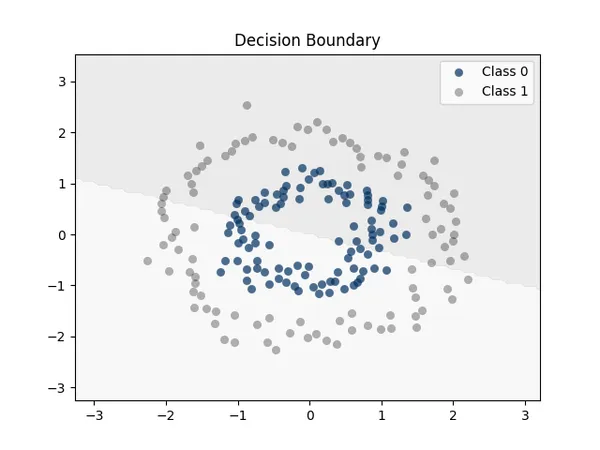
SLP單層模型準確度

Model Accuracy: 50.50%

損失函數

Epoch 10, Loss: 0.7951
Epoch 20, Loss: 0.7521
...
Epoch 90, Loss: 0.6939
Epoch 100, Loss: 0.6935

2. 準備資料階段

使用Numpy的隨機常態分佈來做為簡易資料集，

以下主要任務

• 隨機生成資料各100筆
• 合併資料集
• 繪製資料點視覺化

# %% 資料準備
# 生成環形數據
np.random.seed(40)
n_points = 100

# 類 0: 圓形內部
theta = np.linspace(0, 2 * np.pi, n_points)
r_0 = 1 + 0.2 * np.random.randn(n_points)  # 加一些隨機擾動
class_0 = np.vstack([r_0 * np.cos(theta), r_0 * np.sin(theta)]).T

# 類 1: 圓形外部
r_1 = 2 + 0.2 * np.random.randn(n_points)  # 外圓
class_1 = np.vstack([r_1 * np.cos(theta), r_1 * np.sin(theta)]).T

print("class_0 shape:", class_0[:5], class_0.shape)
print("class_1 shape:", class_0[:5], class_1.shape)
# 合併資料與標籤
data = np.vstack([class_0, class_1]).astype(np.float32)
labels = np.array([0]*100 + [1]*100).astype(np.float32).reshape(-1, 1)

# 顯示合併後資料與 shape
print("Data set:", data[:1], "shape:", data.shape)
print("Labels set:", labels[:1], "shape:", labels.shape)

# 繪製數據
plt.scatter(class_0[:, 0], class_0[:, 1], color='#003060', label='Class 0', alpha=0.7, s=40)
plt.scatter(class_1[:, 0], class_1[:, 1], color='black', label='Class 1', alpha=0.3, s=40)
plt.legend()
plt.title("Circular Data")
plt.show()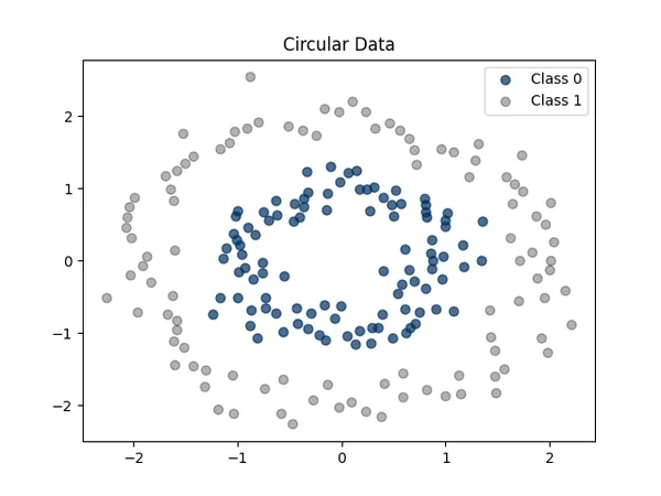

2. 建立多層感知器（Multilayer Perceptron, MLP）

# %% 多層感知器 (Multilayer Perceptron, MLP) 設計
class MultilayerPerceptron:
    def __init__(self, input_dim, hidden_dim):
        # 隱藏層的權重和偏置
        self.W1 = tf.Variable(tf.random.normal([input_dim, hidden_dim]))
        self.b1 = tf.Variable(tf.zeros([hidden_dim]))
        # 輸出層的權重和偏置
        self.W2 = tf.Variable(tf.random.normal([hidden_dim, 1]))
        self.b2 = tf.Variable(tf.zeros([1]))

    def forward(self, x):
        # 隱藏層 + ReLU 激活函數
        hidden_output = tf.nn.relu(tf.matmul(x, self.W1) + self.b1)
        return tf.matmul(hidden_output, self.W2) + self.b2

前向傳播（Forward Propagation）

$$y = f(Wx + b)$$

    def forward(self, x):
        # 隱藏層 + ReLU 激活函數
        hidden_output = tf.nn.relu(tf.matmul(x, self.W1) + self.b1)
        return tf.matmul(hidden_output, self.W2) + self.b2

relu : ReLU激活函數 W1：定義隱藏層矩陣加權，為矩陣乘法運算 b1：平移調整模型的決策邊界，這邊設為0 forward(self, x) : 經過加權後的矩陣，輸出為一個預測值

3. 訓練模型階段

# 定義交叉熵損失函數
def binary_crossentropy_loss(y_true, y_pred):
    return tf.reduce_mean(tf.nn.sigmoid_cross_entropy_with_logits(labels=y_true, logits=y_pred))

# 訓練模型
def train_model(model, data, labels, learning_rate=0.1, epochs=100):
    optimizer = tf.optimizers.SGD(learning_rate)

    loss_history = []
    for epoch in range(epochs):
        with tf.GradientTape() as tape:
            logits = model.forward(data)  # 前向傳播
            loss = binary_crossentropy_loss(labels, logits)  # 計算損失

        # 計算梯度並更新權重
        gradients = tape.gradient(
            loss, [model.W1, model.b1, model.W2, model.b2])  # 更新所有權重和偏置
        optimizer.apply_gradients(
            zip(gradients, [model.W1, model.b1, model.W2, model.b2]))

        # 損失函數變化紀錄
        loss_history.append(loss.numpy())
        if (epoch+1) % 10 == 0:
            print(f"Epoch {epoch+1}, Loss: {loss.numpy():.4f}")

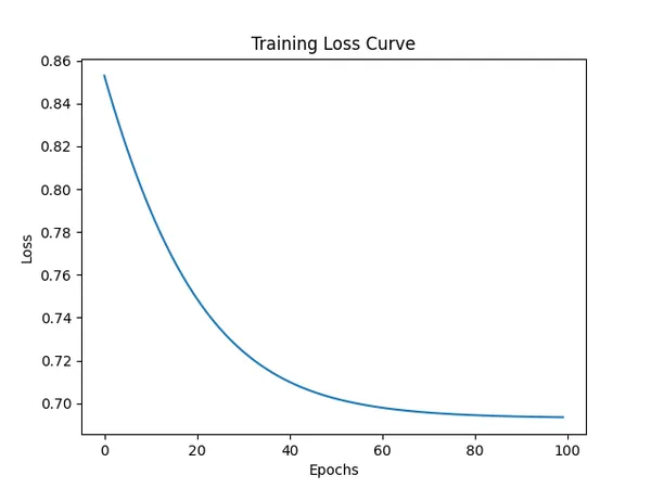
    # 畫出損失曲線
    plt.plot(loss_history)
    plt.xlabel("Epochs")
    plt.ylabel("Loss")
    plt.title("Training Loss Curve")
    plt.show()

    return model

因為使用的是TensorFlow 低階語言，在語法邏輯上會將步驟拆分更細，因此依序做說明。

模型超參數（Hyperparameter）

def train_model(model, data, labels, learning_rate=0.1, epochs=100)

帶入模型、數據集、真實標籤、學習率、訓練次數

計算梯度

with tf.GradientTape() as tape:
		logits = model.forward(data)  
		loss = binary_crossentropy_loss(labels, logits)

1. 向前傳播

使用model.forward 函數來計算預測值，data 是要預測的資料集，經函數加權(weights)後輸出值為 logits

2. 計算損失函數

# 定義二元交叉熵損失函數
def binary_crossentropy_loss(y_true, y_pred):
    return tf.reduce_mean(tf.nn.sigmoid_cross_entropy_with_logits(labels=y_true, logits=y_pred))

tf.nn.sigmoid_cross_entropy_with_logits(labels=y_true, logits=y_pred) : 計算真實標籤與預測值之間的損失數

sigmoid : 此函數使用sigmoid函數來進行二元分類，在使用交叉熵（Cross-Entropy）來計算損失數

loss = binary_crossentropy_loss(labels, logits)  # 計算損失

所以這邊最終獲得了損失數 loss

反向傳播（Backpropagation）

反向傳播主要目的是計算當前梯度，使用微積分中的微分與鏈鎖法則(Chain Rule)概念，在TensorFlow中已經包裝成一個函數可以使用，只需要帶入定義在model中的隱藏層和輸出層即可，也就是前向傳播的路徑

        # 計算梯度並更新權重
        gradients = tape.gradient(
            loss, [model.W1, model.b1, model.W2, model.b2])  # 更新所有權重和偏置

透過鏈鎖法則的數學觀念可以得知，它將原先前向傳播的路徑反方向逐層遞回，並透過偏微分計算出每個參數（如 $W_1$, $b_1$ 等）對整體損失函數 $L$ 的影響程度 對於參數的梯度可以表示為

$$\left[ \frac{\partial L}{\partial W_1}, \frac{\partial L}{\partial b_1}, \frac{\partial L}{\partial W_2}, \frac{\partial L}{\partial b_2}, \dots \right]$$

梯度下降（Gradient Descent）

梯度下降是一種用來最小化損失函數 $L(\theta)$ 的優化演算法。它透過對每個參數求偏導數（即梯度），沿著損失函數下降最快的方向更新參數。

$$\theta := \theta - \alpha \cdot \nabla_{\theta} J(\theta)$$

• $\theta$：參數（例如權重 weight）
• $\alpha$：學習率（Learning Rate），控制每次更新的幅度
• $\nabla_{\theta} J(\theta)$：損失函數的梯度（Gradient），表示函數變化最快的方向

在上一個反向傳播（Backpropagation） 過程中所得出的梯度，將透過學習率來進行參數更新。

$$\nabla_{\theta} J(\theta) = \left[ \frac{\partial L}{\partial W_1},\, \frac{\partial J}{\partial b_1},\, \frac{\partial J}{\partial W_2},\, \frac{\partial J}{\partial b_2} \right]$$

優化器 Optimizer

在TensorFlow中使用物件optimizers，選擇的方法為隨機梯度下降（Stochastic Gradient Descent） 方法，並帶入學習率參數

optimizer.apply_gradients :即為梯度下降函數

    optimizer = tf.optimizers.SGD(learning_rate)
            optimizer.apply_gradients(
            zip(gradients, [model.W1, model.b1, model.W2, model.b2]))

損失函數視覺化

將每一次訓練epochs所計算的損失函數記錄在 list 中

        # 損失函數變化紀錄
        loss_history.append(loss.numpy())
        if (epoch+1) % 10 == 0:
            print(f"Epoch {epoch+1}, Loss: {loss.numpy():.4f}")
    
    # 畫出損失曲線
    plt.plot(loss_history)
    plt.xlabel("Epochs")
    plt.ylabel("Loss")
    plt.title("Training Loss Curve")
    plt.show()

每次訓練中的損失函數

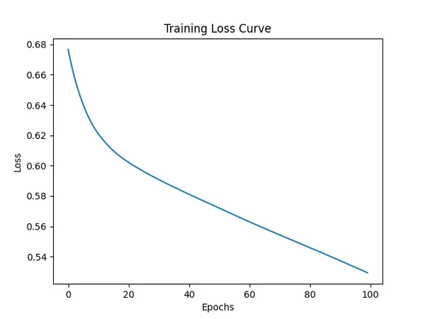
Epoch 10, Loss: 0.6240
Epoch 20, Loss: 0.6035
...
Epoch 90, Loss: 0.5382
Epoch 100, Loss: 0.5294

4. 評估模型階段

def predict(model, data) :
    logits = model.forward(data)
    return tf.sigmoid(logits).numpy() > 0.5

sigmoid函數

特性轉換成 0 或 1，適合二元分類，0.5為中間點邊界，將函數將輸入值趨近於0或1

準確率評估

計算預測函數與實際標籤的正確數與總數，並求出成功機率

def evaluate_accuracy(model, data, labels):
    predictions = predict(model, data)
    accuracy = np.mean(predictions == labels)
    print(f"Model Accuracy: {accuracy * 100:.2f}%")
    return accuracy

評估結果

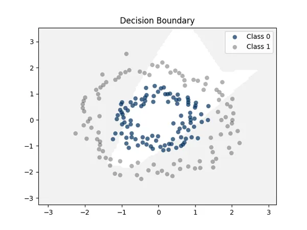
Model Accuracy: 74.00%

5. 視覺化決策邊界

# 視覺化決策邊界
def plot_decision_boundary(model, data, labels):
    x_min, x_max = data[:, 0].min() - 1, data[:, 0].max() + 1
    y_min, y_max = data[:, 1].min() - 1, data[:, 1].max() + 1
    xx, yy = np.meshgrid(np.linspace(x_min, x_max, 100),
                         np.linspace(y_min, y_max, 100))
    grid_data = np.c_[xx.ravel(), yy.ravel()].astype(np.float32)

    # 預測網格點
    predictions = predict(model, grid_data).reshape(xx.shape)

    plt.contourf(xx, yy, predictions, colors=['white', 'gray'], alpha=0.1)
    plt.scatter(class_0[:, 0], class_0[:, 1],
                alpha=0.7,
                linewidth=0.1,
                s=40,
                color='#003060',
                label='Class 0'
                )

    plt.scatter(class_1[:, 0], class_1[:, 1],
                alpha=0.3,
                linewidth=0.1,
                s=40,
                color='black',
                label='Class 1'
                )
    plt.legend()

    plt.title("Decision Boundary")
    plt.show()

6. 運行流程整合

model = MultilayerPerceptron(
    input_dim=2, hidden_dim=5)  # 建立模型，2 個輸入特徵，5 個隱藏層神經元
model = train_model(model, data, labels, learning_rate=0.1, epochs=100)  # 訓練模型
evaluate_accuracy(model, data, labels)  # 計算準確率
plot_decision_boundary(model, data, labels)  # 繪製決策邊界